integration of ODEs + derivatives (directional and adjoint)
Description
INDegrator is a library of IND integration schemes.
They allow you to evaluate the solution \(x(t; x_0, p, q)\) of initial value problems (IVP) of the form
\[\begin{split}\dot x =& f(x, p, q) \\ x(0) =& x_0\end{split}\]where \(\dot x\) denotes the derivative of \(x\) w.r.t. \(t\), and additionally
first-order derivatives
\[\begin{split}\frac{\partial x}{\partial (x_0, p, q)}(t; x_0, p, q) \;, \\\end{split}\]and second-order derivatives of the solution
\[\frac{\partial^2 x}{\partial (x_0, p, q)^2}(t; x_0, p, q)\]in an accurate and efficient way.
The derivatives w.r.t. \(x_0\), \(p\) and \(q\) are computed based on the IND and automatic differentiation (AD) principles. Both forward and reverse/adjoint mode computations are supported.
Rationale
- For optimal control (direct approach) one requires accurate derivatives of the solution w.r.t. controls
q.- For least-squares parameter estimation algorithms one requires derivatives of the solution w.r.t. parameters
p.- For experimental design optimization one requires accurate second-order derivatives of the solution w.r.t.
pandq
Features
Explicit Euler, fixed stepsize
- first-order forward
- second-order forward
- first-order reverse
Runge Kutta 4 (RK4), fixed stepsize
- first-order forward
- second-order forward
- first-order reverse
Example
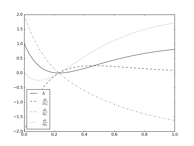
Consider the initial value problem
and the model response function
We would like to compute the derivatives
for \(t_i = \frac{i}{99}, i=0,\dots,99\), \(x_0=2\), \(p=(3,4)\). The following code shows how to setup this task with MSOBox.
import numpy as np
import matplotlib.pyplot as pl
from msobox.ind.rk4classic import RK4Classic


class MF(object):
    def ffcn(self, f, t, x, p, u):
        f[0] = - p[0]*(x[0] - p[1])

    def ffcn_dot(self, f, f_d, t, x, x_d, p, p_d, u, u_d):
        f[0] = - p[0]*(x[0] - p[1])
        f_d[0,:] = -p_d[0,:]*(x[0] - p[1]) \
                     + p[0]*p_d[1,:] \
                     - p[0]*x_d[0,:]

    def hfcn(self, h, t, x, p, u):
        h[0] = (x[0]-p[0])**2

    def hfcn_dot(self, h, h_d, t, x, x_d, p, p_d, u, u_d):
        h[0] = (x[0]-p[0])**2
        h_d[...] = 2.*(x[0]-p[0])*(x_d[0, :] - p_d[0, :])


mf = MF()
ind = RK4Classic(mf)

# initial values and parameters
xp = np.array([2., 3., 4.])
x  = xp[:1]
p  = xp[1:]
q = np.zeros(0)

# time grid and measurement responses
NTS = 100
ts   = np.linspace(0, 1, 100)
hs   = np.zeros((100, 1))

# setup directional derivatives
P   = 3
hs_d = np.zeros((100, 1, P))
xp_d = np.zeros( xp.shape + (P,))
xp_d = np.eye(xp.size)
x_d  = xp_d[:1, :]
p_d  = xp_d[1:, :]
q_d = np.zeros( q.shape + (P,))

# solve initial value problem
for i in range(ts.size-1):
    mf.hfcn_dot(hs[i, ...], hs_d[i, ...], ts[i],x, x_d, p, p_d, q, q_d)
    x[:], x_d[...] = ind.fo_forward(ts[i:i+2], x, x_d, p, p_d, q, q_d)
i = ts.size - 1
mf.hfcn_dot(hs[i, ...], hs_d[i, ...], ts[i],x, x_d, p, p_d, q, q_d)

# plot result
pl.plot(ts, hs[:, 0], '-k', label='$h$')
pl.plot(ts, hs_d[:, 0, 0], '--k', label=r'$\frac{dh}{dx_0}$')
pl.plot(ts, hs_d[:, 0, 1], '-.k', label=r'$\frac{dh}{dp_1}$')
pl.plot(ts, hs_d[:, 0, 2], ':k', label=r'$\frac{dh}{dp_2}$')
pl.legend(loc='best')
pl.savefig('ind.png')
pl.show()